MobileFormer#
在本节中,将介绍一种新的网络-MobileFormer,它实现了 Transformer 全局特征与 CNN 局部特征的融合,在较低的成本内,创造一个高效的网络。通过本节,让大家去了解如何将 CNN 与 Transformer 更好的结合起来,同时实现模型的轻量化。
MobileFormer#
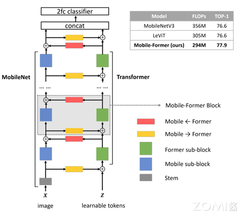
MobileFormer:一种通过双线桥将 MobileNet 和 Transformer 并行的结构。这种方式融合了 MobileNet 局部性表达能力和 Transformer 全局表达能力的优点,这个桥能将局部性和全局性双向融合。和现有 Transformer 不同,Mobile-Former 使用很少的 tokens(例如 6 个或者更少)随机初始化学习全局先验,计算量更小。
并行结构#
Mobile-Former 将 MobileNet 和 Transformer 并行化,并通过双向交叉注意力连接(下见图)。Mobile(指 MobileNet)采用图像作为输入(\(X\in R^{HW \times 3}\)),并应用反向瓶颈块提取局部特征。Former(指 Transformers)将可学习的参数(或 tokens)作为输入,表示为 \(Z\in R^{M\times d}\),其中 M 和 d 分别是 tokens 的数量和维度,这些 tokens 随机初始化。与视觉 Transformer(ViT)不同,其中 tokens 将局部图像 patch 线性化,Former 的 tokens 明显较少(M≤6),每个代表图像的全局先验知识。这使得计算成本大大降低。
低成本双线桥#
Mobile 和 Former 通过双线桥将局部和全局特征双向融合。这两个方向分别表示为 Mobile→Former 和 Mobile←Former。我们提出了一种轻量级的交叉注意力模型,其中映射(\(W^{Q}\),\(W^{K}\),\(W^{V}\))从 Mobile 中移除,以节省计算,但在 Former 中保留。在通道数较少的 Mobile 瓶颈处计算交叉注意力。具体而言,从局部特征图 X 到全局 tokens Z 的轻量级交叉注意力计算如下:
其中局部特征 X 和全局 tokens Z 被拆分进入 h 个头,即 \(X=[\widetilde{x_{1}}...\widetilde{x_{h}}],Z=[\widetilde{z_{1}}...\widetilde{z_{h}}]\) 表示多头注意力。第 i 个头的拆分 \(\widetilde{z_{1}}\in R^{M \times \frac {d}{h} }\) 与第 i 个 token\(\widetilde{z_{1}}\in R^{d}\) 不同。\(W_{i}^{Q}\) 是第 i 个头的查询映射矩阵。\(W^{O}\) 用于将多个头组合在一起。Attn(Q,K,V)是查询 Q、键 K 和值 V 的标准注意力函数,即 :
其中 \([.]_{1:h}\) 表示将 h 个元素 concat 到一起。需要注意的是,键和值的映射矩阵从 Mobile 中移除,而查询的映射矩阵 \(W_{i}^{Q}\) 在 Former 中保留。类似地从全局到局部的交叉注意力计算如下: $\( A_{Z->X} = [Attn(\widetilde{x_{i}},\widetilde{z_{i}}\odot W_{i}^{K},\widetilde{z_{i}}\odot W_{i}^{V})]_{i=1:h}\tag{2} \)$
其中 \(W_{i}^{K}\) 和 \(W_{i}^{V}\) 分别是 Former 中键和值的映射矩阵。而查询的映射矩阵从 Mobile 中移除。
Mobile-Former 块#
Mobile-Former 由 Mobile-Former 块组成。每个块包含四部分:Mobile 子块、Former 子块以及双向交叉注意力 Mobile←Former 和 Mobile→Former(如下图所示)。
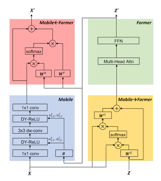
输入和输出:Mobile-Former 块有两个输入:(a) 局部特征图 \(X\in R^{HW\times C}\),为 C 通道、高度 H 和宽度 W,以及(b) 全局 tokens \(Z\in R^{M\times d}\),其中 M 和 d 是分别是 tokens 的数量和维度,M 和 d 在所有块中一样。Mobile-Former 块输出更新的局部特征图 \(X\) 和全局 tokens\(Z\),用作下一个块的输入。
Mobile 子块:如上图所示,Mobile 子块将特征图 \(X\) 作为输入,并将其输出作为 Mobile←Former 的输入。这和反向瓶颈块略有不同,其用动态 ReLU 替换 ReLU 作为激活函数。不同于原始的动态 ReLU,在平均池化特征图上应用两个 MLP 以生成参数。我们从 Former 的第一个全局 tokens 的输出 \(z'_{1}\) 应用两个 MLP 层(上图中的θ)保存平均池化。其中所有块的 depth-wise 卷积的核大小为 3×3。
代码
class Mobile(nn.Module):

    def __init__(self, in_channel, expand_size, out_channel, token_demension, kernel_size=3, stride=1, k=2):
        super(Mobile, self).__init__()
        self.in_channel, self.expand_size, self.out_channel = in_channel, expand_size, out_channel
        self.token_demension, self.kernel_size, self.stride, self.k = token_demension, kernel_size, stride, k

        if stride == 2:
            self.strided_conv = nn.Sequential(
                nn.Conv2d(self.in_channel, self.expand_size, kernel_size=3, stride=2, padding=int(self.kernel_size // 2), groups=self.in_channel).cuda(),
                nn.BatchNorm2d(self.expand_size).cuda(),
                nn.ReLU6(inplace=True).cuda()
            )
            self.conv1 = nn.Conv2d(self.expand_size, self.in_channel, kernel_size=1, stride=1).cuda()
            self.bn1 = nn.BatchNorm2d(self.in_channel).cuda()
            self.ac1 = DynamicReLU(self.in_channel, self.token_demension, k=self.k).cuda()
            self.conv2 = nn.Conv2d(self.in_channel, self.expand_size, kernel_size=3, stride=1, padding=1, groups=self.in_channel).cuda()
            self.bn2 = nn.BatchNorm2d(self.expand_size).cuda()
            self.ac2 = DynamicReLU(self.expand_size, self.token_demension, k=self.k).cuda()
            self.conv3 = nn.Conv2d(self.expand_size, self.out_channel, kernel_size=1, stride=1).cuda()
            self.bn3 = nn.BatchNorm2d(self.out_channel).cuda()
        else:
            self.conv1 = nn.Conv2d(self.in_channel, self.expand_size, kernel_size=1, stride=1).cuda()
            self.bn1 = nn.BatchNorm2d(self.expand_size).cuda()
            self.ac1 = DynamicReLU(self.expand_size, self.token_demension, k=self.k).cuda()
            self.conv2 = nn.Conv2d(self.expand_size, self.expand_size, kernel_size=3, stride=1, padding=1, groups=self.expand_size).cuda()
            self.bn2 = nn.BatchNorm2d(self.expand_size).cuda()
            self.ac2 = DynamicReLU(self.expand_size, self.token_demension, k=self.k).cuda()
            self.conv3 = nn.Conv2d(self.expand_size, self.out_channel, kernel_size=1, stride=1).cuda()
            self.bn3 = nn.BatchNorm2d(self.out_channel).cuda()

    def forward(self, x, first_token):
        if self.stride == 2:
            x = self.strided_conv(x)
        x = self.bn1(self.conv1(x))
        x = self.ac1(x, first_token)
        x = self.bn2(self.conv2(x))
        x = self.ac2(x, first_token)
        return self.bn3(self.conv3(x))
Former 子块:Former 子块是一个标准的 Transformer 块,包括一个多头注意力(MHA)和一个前馈网络(FFN)。在 FFN 中,膨胀率为 2(代替 4)。使用 post 层归一化。Former 在 Mobile→Former 和 Mobile←Former 之间处理(见上图)。
代码
class Former(nn.Module):

    def __init__(self, head, d_model, expand_ratio=2):
        super(Former, self).__init__()
        self.d_model = d_model
        self.expand_ratio = expand_ratio
        self.eps = 1e-10
        self.head = head
        assert self.d_model % self.head == 0
        self.d_per_head = self.d_model // self.head

        self.QVK = MLP([self.d_model, self.d_model * 3], bn=False).cuda()
        self.Q_to_heads = MLP([self.d_model, self.d_model], bn=False).cuda()
        self.K_to_heads = MLP([self.d_model, self.d_model], bn=False).cuda()
        self.V_to_heads = MLP([self.d_model, self.d_model], bn=False).cuda()
        self.heads_to_o = MLP([self.d_model, self.d_model], bn=False).cuda()
        self.norm = nn.LayerNorm(self.d_model).cuda()
        self.mlp = MLP([self.d_model, self.expand_ratio * self.d_model, self.d_model], bn=False).cuda()
        self.mlp_norm = nn.LayerNorm(self.d_model).cuda()

    def forward(self, x):
        QVK = self.QVK(x)
        Q = QVK[:, :, 0: self.d_model]
        Q = rearrange(self.Q_to_heads(Q), 'n m ( d h ) -> n m d h', h=self.head)
        K = QVK[:, :, self.d_model: 2 * self.d_model]
        K = rearrange(self.K_to_heads(K), 'n m ( d h ) -> n m d h', h=self.head)
        V = QVK[:, :, 2 * self.d_model: 3 * self.d_model]
        V = rearrange(self.V_to_heads(V), 'n m ( d h ) -> n m d h', h=self.head)
        scores = torch.einsum('nqdh, nkdh -> nhqk', Q, K) / (np.sqrt(self.d_per_head) + self.eps)
        scores_map = F.softmax(scores, dim=-1)
        v_heads = torch.einsum('nkdh, nhqk -> nhqd', V, scores_map)
        v_heads = rearrange(v_heads, 'n h q d -> n q ( h d )')
        attout = self.heads_to_o(v_heads)
        attout = self.norm(attout)
        attout = self.mlp(attout)
        attout = self.mlp_norm(attout)
        return attout
Mobile→Former:文章提出的轻量级交叉注意力(式 1)用于将局部特征 X 融合到全局特征 tokens Z。与标准注意力相比,映射矩阵的键 \(W^{K}\) 和值 \(W^{V}\)(在局部特征 X 上)被移除以节省计算(见上图)。
代码
class Mobile_Former(nn.Module):
    '''局部特征 -> 全局特征'''
    def __init__(self, d_model, in_channel):
        super(Mobile_Former, self).__init__()
        self.d_model, self.in_channel = d_model, in_channel

        self.project_Q = nn.Linear(self.d_model, self.in_channel).cuda()
        self.unproject = nn.Linear(self.in_channel, self.d_model).cuda()
        self.eps = 1e-10
        self.shortcut = nn.Sequential().cuda()

    def forward(self, local_feature, x):
        _, c, _, _ = local_feature.shape
        local_feature = rearrange(local_feature, 'n c h w -> n ( h w ) c')
        project_Q = self.project_Q(x)
        scores = torch.einsum('nmc , nlc -> nml', project_Q, local_feature) * (c ** -0.5)
        scores_map = F.softmax(scores, dim=-1)
        fushion = torch.einsum('nml, nlc -> nmc', scores_map, local_feature)
        unproject = self.unproject(fushion)
        return unproject + self.shortcut(x)
Mobile←Former:这里的交叉注意力(式 2)与 Mobile→Former 的方向相反,其将全局 tokens 融入本地特征。局部特征是查询,全局 tokens 是键和值。因此,我们保留键 \(W^{K}\) 和值 \(W^{V}\) 中的映射矩阵,但移除查询 \(W^{Q}\) 的映射矩阵以节省计算,如上图所示。
计算复杂度:Mobile-Former 块的四个核心部分具有不同的计算成本。给定输入大小为 \(HW\times C\) 的特征图,以及尺寸为 d 的 M 个全局 tokens,Mobile 占据了大部分的计算量 \(O(HWC^{2})\)。Former 和双线桥是重量级的,占据不到总计算成本的 20%。具体而言,Former 的自注意力和 FFN 具有复杂度 \(O(M^{2}d+Md^{2})\)。Mobile→Former 和 Mobile←Former 共享交叉注意力的复杂度 \(O(MHWC+MdC)\)。
代码
class Former_Mobile(nn.Module):
    '''全局特征 -> 局部特征'''
    def __init__(self, d_model, in_channel):
        super(Former_Mobile, self).__init__()
        self.d_model, self.in_channel = d_model, in_channel

        self.project_KV = MLP([self.d_model, 2 * self.in_channel], bn=False).cuda()
        self.shortcut = nn.Sequential().cuda()

    def forward(self, x, global_feature):
        res = self.shortcut(x)
        n, c, h, w = x.shape
        project_kv = self.project_KV(global_feature)
        K = project_kv[:, :, 0 : c]
        V = project_kv[:, :, c : ]
        x = rearrange(x, 'n c h w -> n ( h w ) c')
        scores = torch.einsum('nqc, nkc -> nqk', x, K)
        scores_map = F.softmax(scores, dim=-1)
        v_agg = torch.einsum('nqk, nkc -> nqc', scores_map, V)
        feature = rearrange(v_agg, 'n ( h w ) c -> n c h w', h=h)
        return feature + res
网络结构#
一个 Mobile-Former 架构,图像大小为 224×224,294M FLOPs,以不同的输入分辨率堆叠 11 个 Mobile-Former 块。所有块都有 6 个维度为 192 的全局 tokens。它以一个 3×3 的卷积作为 stem 和第一阶段的轻量瓶颈块,首先膨胀,然后通过 3×3 depth-wise 卷积和 point-wise 卷积压缩通道数。第 2-5 阶段包括 Mobile-Former 块。每个阶段的下采样,表示为 Mobile-Former 分类头在局部特征应用平均池化,首先和全局 tokens concat 到一起,然后经过两个全连接层,中间是 h-swish 激活函数。Mobile-Former 有七种模型,计算成本从 26M 到 508M FLOPs。它们的结构相似,但宽度和高度不同。
代码
class MobileFormerBlock(nn.Module):
    def __init__(self, in_channel, expand_size, out_channel, d_model, stride=1, k=2, head=8, expand_ratio=2):
        super(MobileFormerBlock, self).__init__()

        self.in_channel, self.expand_size, self.out_channel = in_channel, expand_size, out_channel
        self.d_model, self.stride, self.k, self.head, self.expand_ratio = d_model, stride, k, head, expand_ratio

        self.mobile = Mobile(self.in_channel, self.expand_size, self.out_channel, self.d_model, kernel_size=3, stride=self.stride, k=self.k).cuda()
        self.former = Former(self.head, self.d_model, expand_ratio=self.expand_ratio).cuda()
        self.mobile_former = Mobile_Former(self.d_model, self.in_channel).cuda()
        self.former_mobile = Former_Mobile(self.d_model, self.out_channel).cuda()

    def forward(self, local_feature, global_feature):
        z_hidden = self.mobile_former(local_feature, global_feature)
        z_out = self.former(z_hidden)
        x_hidden = self.mobile(local_feature, z_out[:, 0, :])
        x_out = self.former_mobile(x_hidden, z_out)
        return x_out, z_out
小结与思考#
本文提出了一种基于 MobileNet 和 Transformer 的双向式交互并行设计的网络 Mobile-Former。它利用了 MobileNet 在局部信息处理中的效率和 Transformer 在编码全局交互方面的优势。该设计不仅有效地提高了计算精度,而且还有效地节省了计算成本。在低 FLOP 条件下,它在图像分类和目标检测方面都优于高效的 CNN 和 ViT 变体。